Numerical integration
When to use numerical integration?
- when you can't integrate analytically (99% of the real life case)
- when a numerical solution is all we need and analytically integrating is hard
- when there is no analytical source
- integrate power consumption of a piece of equipment
- calculate volume of a complicated object
Method
Start from the mathematical definition and split into $N$ intervals
$$ \int_a^b f(x) dx = \sum_{i=0}^{N-1} \int\limits_{x_i}^{x_{i+1}} f(x) dx $$we have $x_0=a$, $x_N=b$.
We define $\Delta x = \frac{b-a}{N}$.
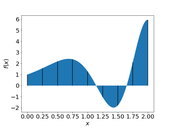
If panels are narrow enough we can approximate the function inside the panel $i$:
$$ f(x) = f(x_i) + f^\prime(x_i) h + \frac12f^{\prime\prime}(x_i) h^2 +... $$with $h = x-x_i$.
We can now devise different integration methods with differring degree of precision by including more of fewer terms in the expansion.
Rectangle method
For the rectangle method we only take the first term:
$$ \int_a^b f(x) dx = \sum_{i=0}^{N-1} \int\limits_{x_i}^{x_{i+1}} f(x_i)dx \approx \frac{b-a}{N}\sum_{i=0}^{N-1}f(x_i) $$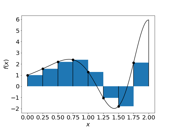
We can also expand the function from the right boundary of each panel and we get
$$ \int_a^b f(x) dx \approx \sum_{i=0}^{N-1} \int\limits_{x_i}^{x_{i+1}} f(x_i) dx \approx \frac{b-a}{N}\sum_{i=1}^{N}f(x_i) $$$$= \Delta x \sum\limits_{i=1}^{N}f(x_i)$$| right rectangles | left rectangles |
|---|---|
 |
|
Or we can expand around the middle of the interval:
$$ \int_a^b f(x) dx = \sum_{i=0}^{N-1} \int\limits_{x_i}^{x_{i+1}} f(m_i) dx \approx \frac{b-a}{N}\sum_{i=1}^{N}f(m_i) = \Delta x \sum_{i=1}^{N}f(m_i) $$where
$$m_i = \frac{x_i+x_{i-1}}{2}$$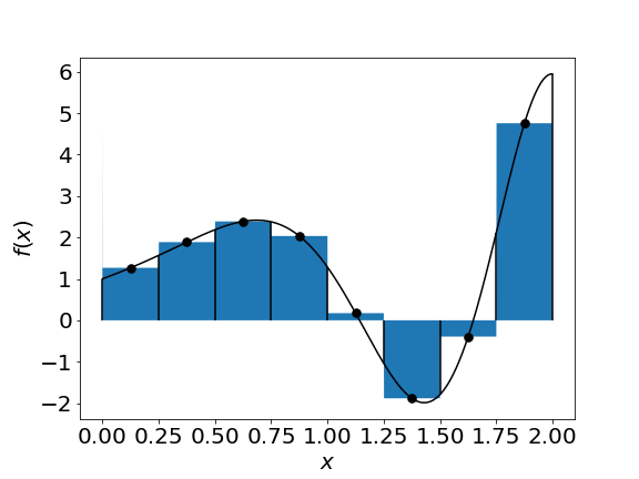
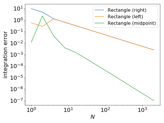
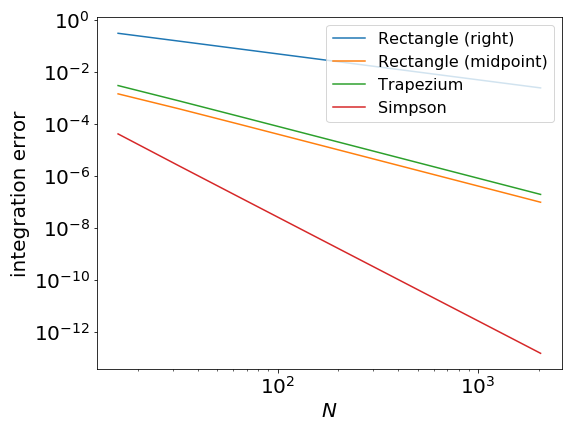
Error estimate
In "normal" conditions the error scales with increasing number of panels $N$ as
- $N^{-1}$ for the left- or right-rectangle method
- $N^{-2}$ for the midpoint method
Trapezium rule
We can improve the situation by increasing the order of the approximation. If we include the first derivative information we obtain the trapezium rule, which approximates the curve with linear segments:

Derivation
$$ \int_a^b f(x) dx \approx \sum_{i=0}^{N-1} \int\limits_{x_i}^{x_{i+1}} f(x_i)+ (x-x_i)\frac{f(x_{i+1})-f(x_i)}{x_{i+1}-x_1} $$$$ = \sum_{i=0}^{N-1} \left( \Delta x f(x_i) + \frac{1}{2}\Delta x^2\frac{f(x_{i+1})-f(x_i)}{\Delta x}\right) $$$$ = \sum_{i=0}^{N-1} \Delta x \frac12 \left( f(x_i)+f(x_{i+1}) \right) =\Delta x\left[\sum_{i=1}^{N-1}f(x_i) +\frac12\left(f(a)+f(b)\right)\right]$$Cost
- requires $N+1$ function evaluation
- one more than the rectangle method
- error scales like $N^{-2}$
Error estimate

Simpson Rule
- For each panel we can approximate the function by a quadratic function.
- we need three points for each panel
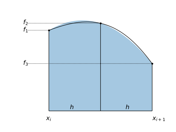
Derivation
Ansatz:
$$g(x)=a x^2 + bx +c$$Solve equations
$ g(0) = f_1 $,
$ g(h) = f_2 $,
$ g(2h) = f_3 $ for $a$, $b$, $c$
Integrate $g(x)$ over the interval $[0,2h]$ gives:
$$ \frac{h}{3}\left(f_1+4f_2+f_3\right) = \Delta x\frac{1}{6}\left(f_1+4f_2+f_3\right). $$import sympy
x, h, f1, f2, f3 = sympy.symbols("x h f1 f2 f3")
a, b, c = sympy.symbols("a b c")
def g(x):
return a*x**2 + b*x + c
abcRule = sympy.solve([
g(0) - f1,
g(h) - f2,
g(2 * h) - f3,
],a,b,c)
integ = sympy.integrate(g(x) , (x , 0, 2*h ) )
integ.subs(abcRule).simplify()
Now combine all panels:
$$ \int_a^b f(x) dx \approx \frac{ \Delta x}{6} \bigg( f(x_0) + 4 f(m_1) + 2 f(x_1) + 4 f(m_2) + 2 f(x_2) + ... + 4 f(m_{N-1})+ 2 f(x_{N-1})+ 4 f(m_{N})+ f(x_N) \bigg)$$Error estimate
Higher order approximation
- we can use higher and higher order approximations
- faster convergence for smooth functions
- numerical round-off issues

Validity
- Higher order only helps if the function and its derivatives are smooth
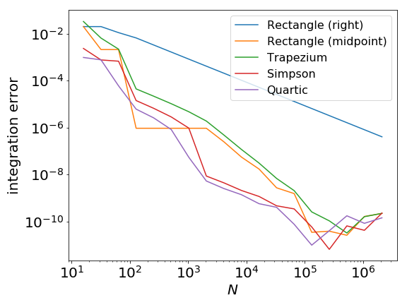
- Only help if there are no divergences

- a too high order approximation can be less optimal if the function being integrated is not of high order
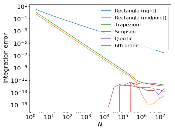
Comparison table
This table shows the number of function evaluations and the asymptotic behaviour of the integration error (under appropriate smoothness condition) for the methods we have seen in this lecture.
| method | # function evaluation | error |
|---|---|---|
| Rectangle | $N$ | $N^{-1}$ |
| Mid-point | $N$ | $N^{-2}$ |
| Trapezium | $N+1$ | $N^{-2}$ |
| Simpson | $2N+1$ | $N^{-4}$ |
| Quartic | $4N+1$ | $N^{-6}$ |
| 6th order | $6N+1$ | $N^{-8}$ |
N.B. This is for single variable integrals, it gets worse as the number of variables increases.
Assignment 2
You should now be able to start the second assignment which investigates numerical integration using Simpson's rule.