First order ODE
ODEs
An ordinary differential equation is an equation of the form
$$G(t,x(t),x'(t),x''(t),...)=0$$
- It is called first order if only $x$ and $x'$ appear in $G$.
- a first order ODE is called explicit if one can write it as
$$ x'(t) = f(x(t),t)$$
Differential equation applications
Differential equations describe the dynamics of many systems:
- Physics:
- ballistics, planets and spacecrafts trajectories (Newton's law)
- fluid dynamics (Navier-Stokes equation)
- Electromagnetism (Maxwell's equations)
- General relativity (Einstein's field equation)
- Thermodynamics
- Chemistry
- Biology
- Economics
In most cases the equations cannot be solved analytically: we need numerical methods.
ODE vs integration
Integration and ODEs are related.
Integration: $$ \frac{dx}{dt} = f(t)$$
Differential equation: $$ \frac{dx}{dt} = f(x(t),t)$$
An ODE where $f$ does not depend on $x(t)$ is an integration.
Euler method
Consider explicit case where we can write
$$ \frac{dx}{dt}=f(x(t),t)$$
We start from the usual place: the definition of the derivative.
$$ \frac{dx}{dt} = \lim_{\Delta t\rightarrow 0} \frac{x(t+\Delta t)-x(t)}{\Delta t}$$
Solve for $x(t+\Delta t)$:
$$ x(t+\Delta t) \approx x(t) + \Delta t \frac{dx}{dt} = x(t) + \Delta t f(x(t),t) $$
Example: Radioactive decay
- A population of unstable nuclei undergoes radioactive decay
- A single nuclei decays at a random time
- The ‘continuum behaviour’ of this random process can be described by an ODE
- continuum means we treat the number of nuclei as a real number instead of an integer
- statistically meaningful but not realistic for a single experiment
Number of nuclei at time $t_0$: $N_0$
Mean lifetime of the decay process: $\tau$
Differential equation:
$$ \frac{dN}{dt} = - \frac{N(t)}{\tau}\equiv f(N,t)$$
Analytical solution:
$$ N(t)= N_0 e^{-t/\tau} $$
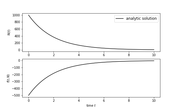
With the analytical solution we can relate the derivative and the number of nuclei:

The area under the curve is the change in the number of nuclei.
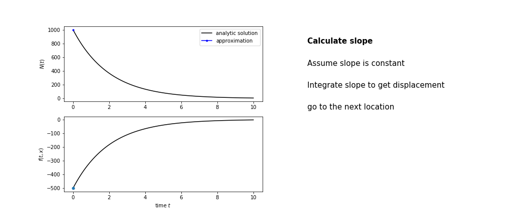
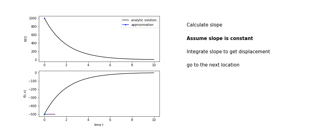
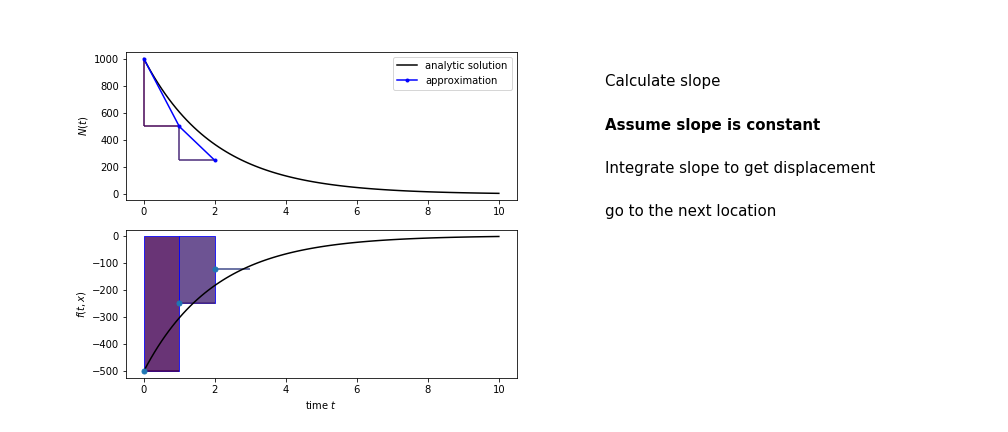
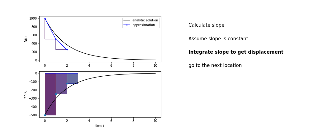
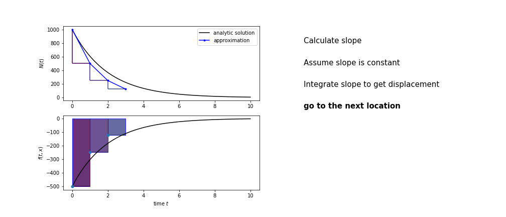
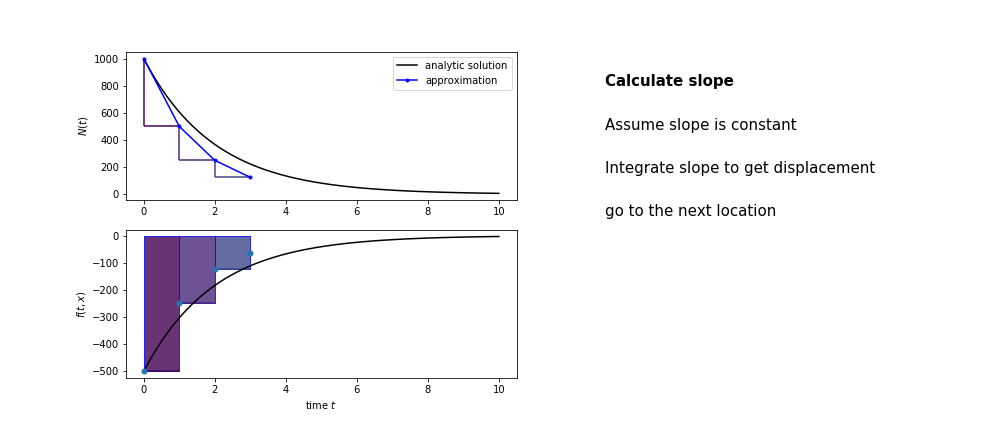
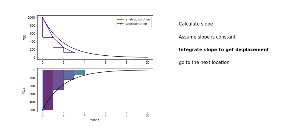
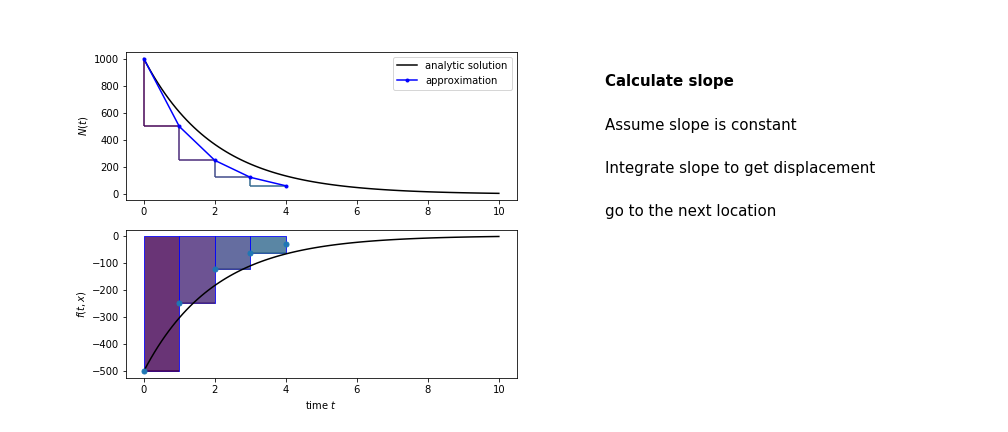
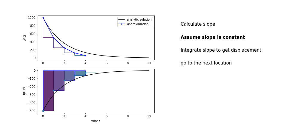
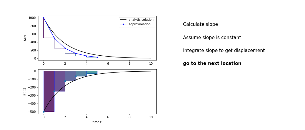
If we do not know the analytical solution things get more complicated, we need to:
- know $N$ to calculate the derivative
- know the derivative to calculate the next position
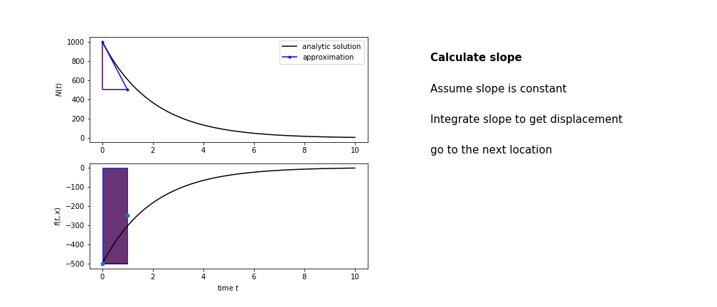
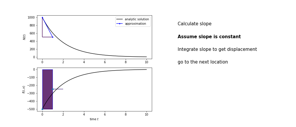
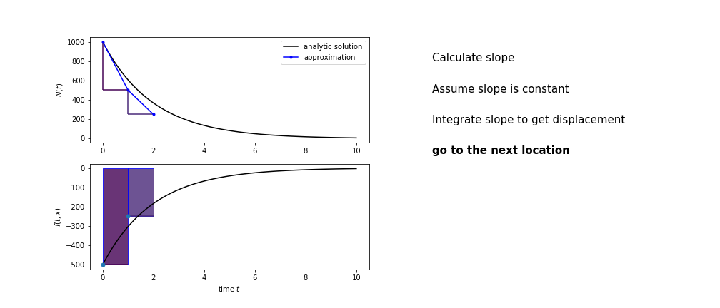
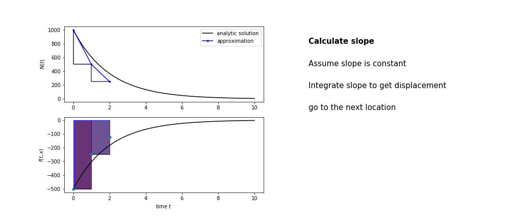
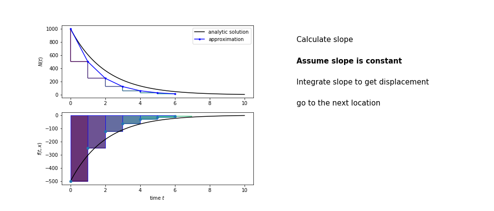
So we get the algorithm
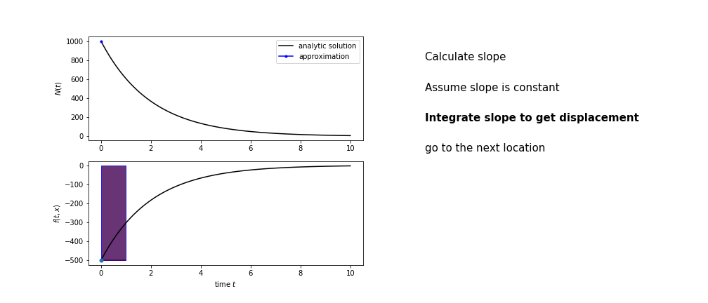
- estimate the area under the derivative for a small step
- change position according to this area
- repeat
Different methods have different ways of estimating the area under the derivative curve. Euler's method estimates the area under the derivative using the rectangle method
| order | integration method | ODE method |
|---|---|---|
| 0 | Rectangle | Euler |
| 1 | Trapezium rule | Heun |
| 2 | Simpson rule | Runge Kutta 4 |
Euler's method demo


Assignment 3
You can now do the first part of assignment 3 which looks at radioactive decay using Euler's method.
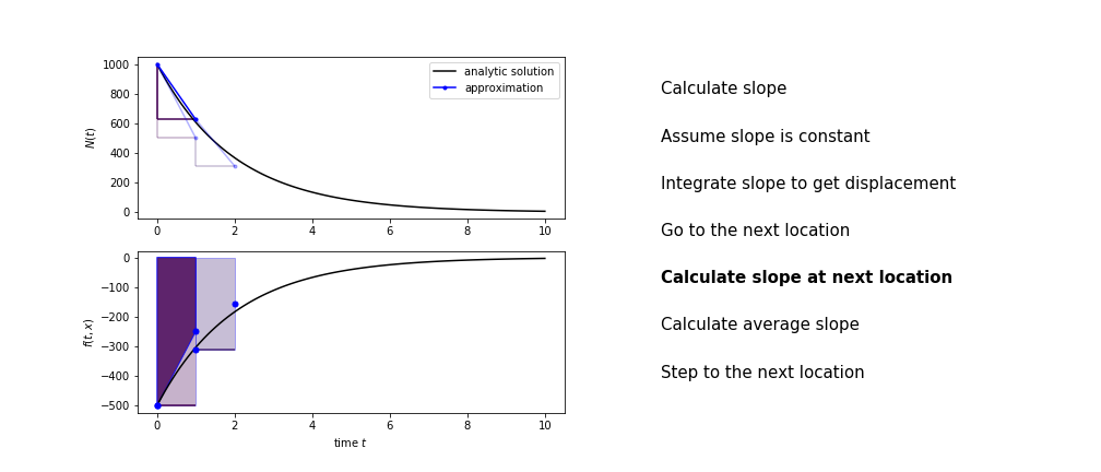
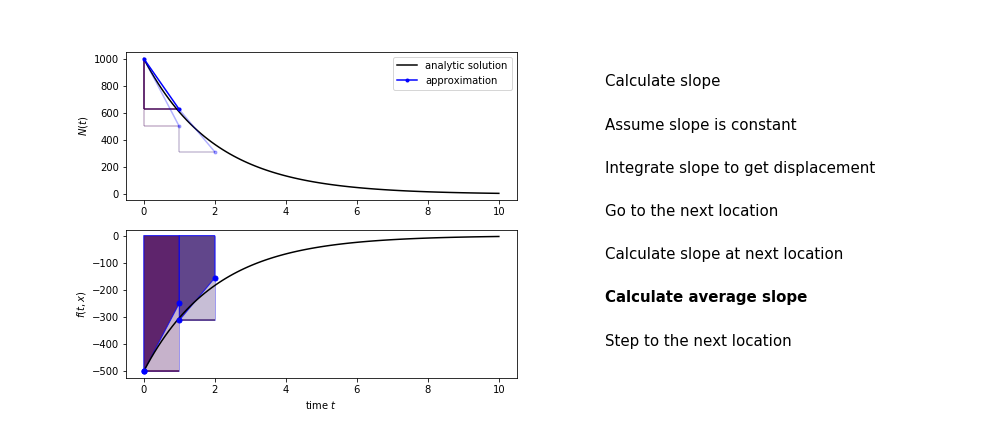
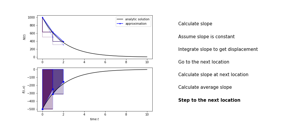
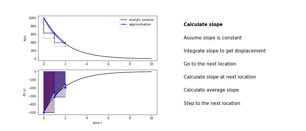
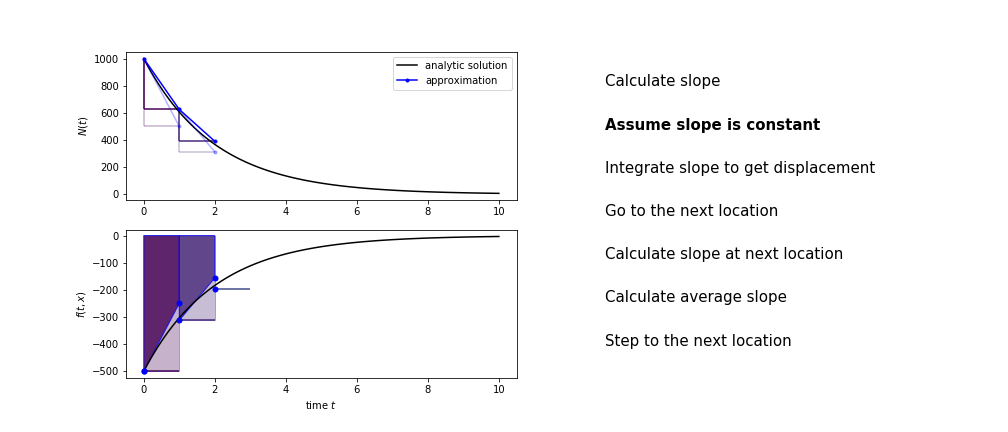
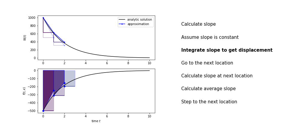
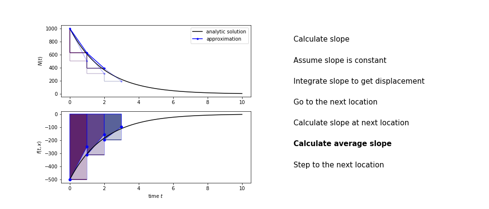
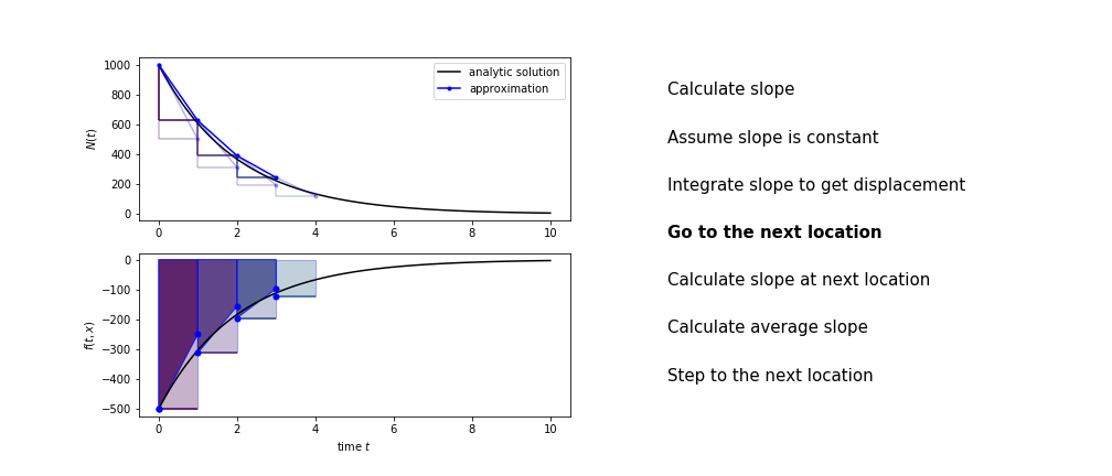
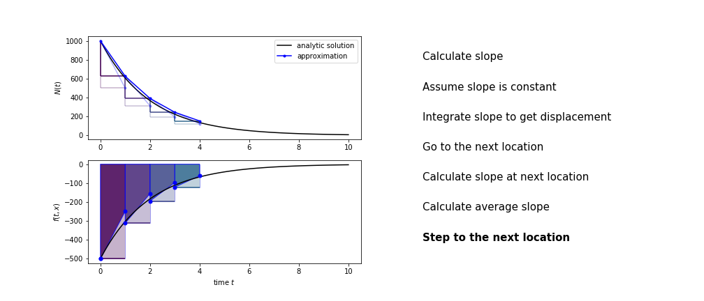
Heun's method
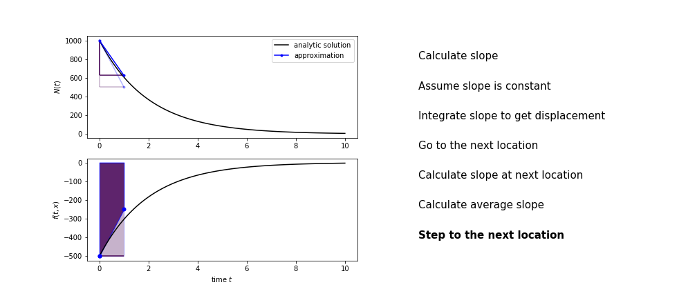
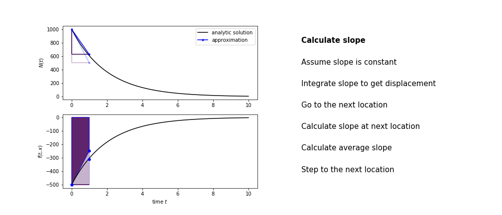
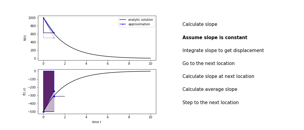
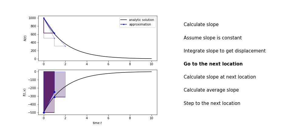
Heun's method uses the same idea than the trapezium method to improve the estimate of the area under the derivative curve.
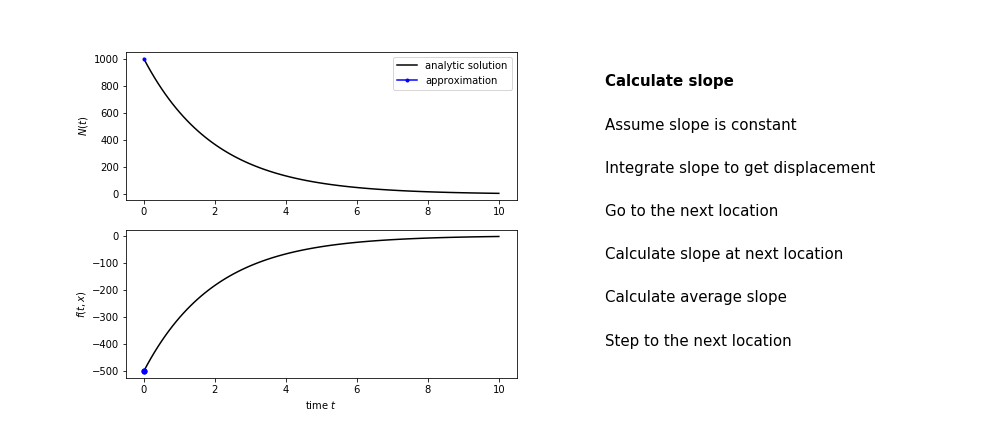
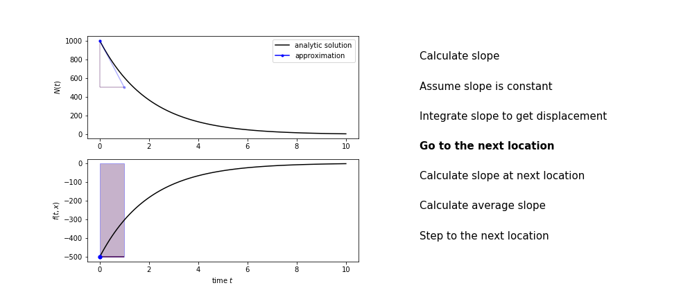
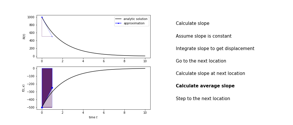
The algorithm is:
- use the slope at the current point to jump to the next point
- calculate the slope there
- use the average of the two slopes to advance
Heun's method demo


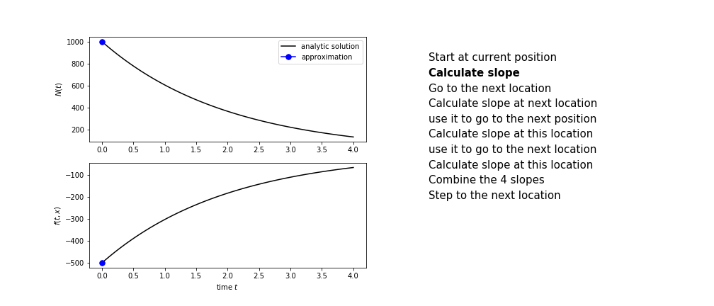
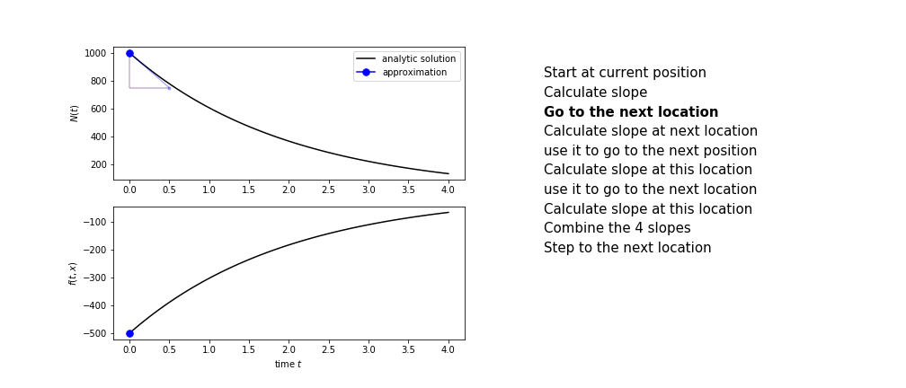
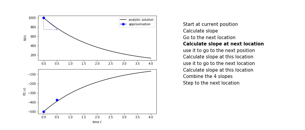
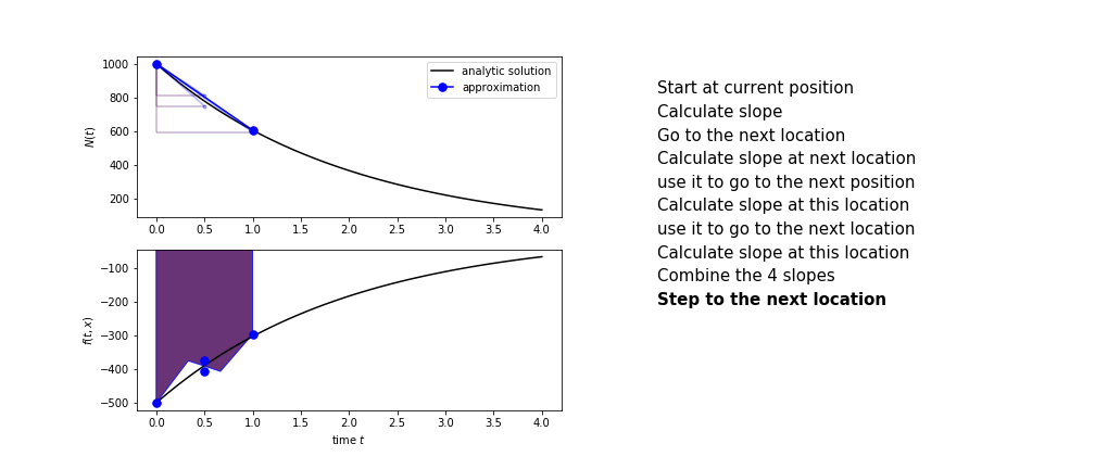
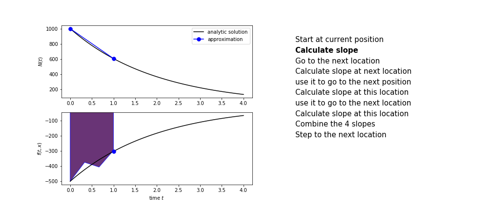
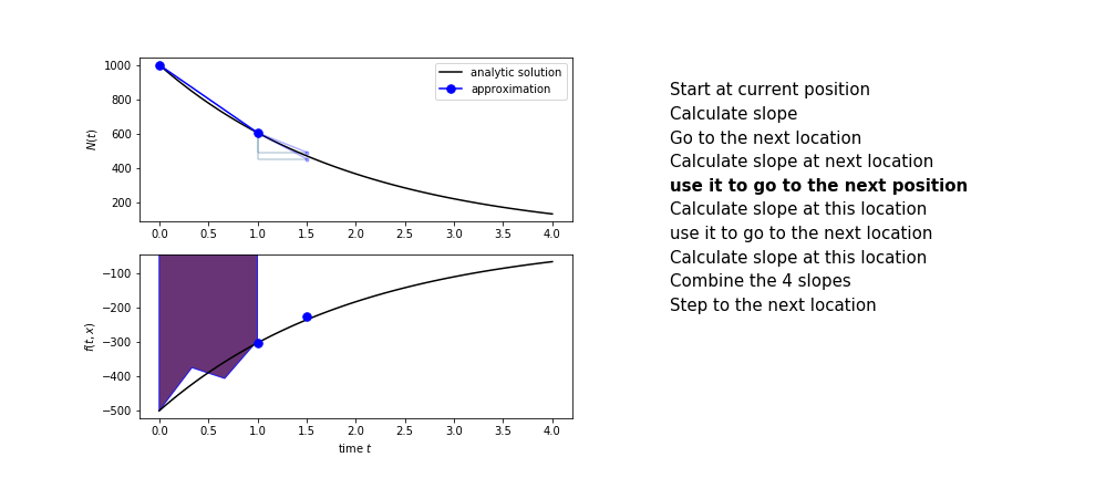
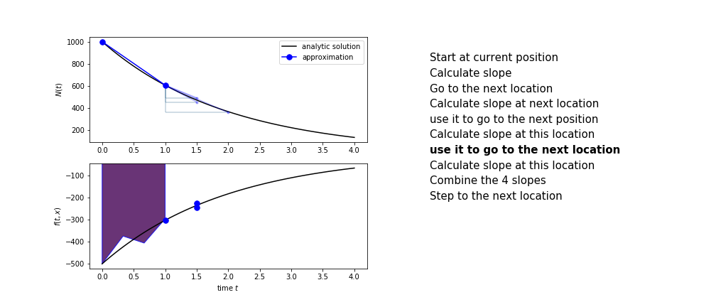
Runge Kutta
Heun's method is one of the Runge Kutta family of methods that use multiple intermediate steps to determine the value of the function after a time step.
The most used is one involving four intermediate steps, it is called Runge-Kutta 4 but is it often simply named "Runge-Kutta"
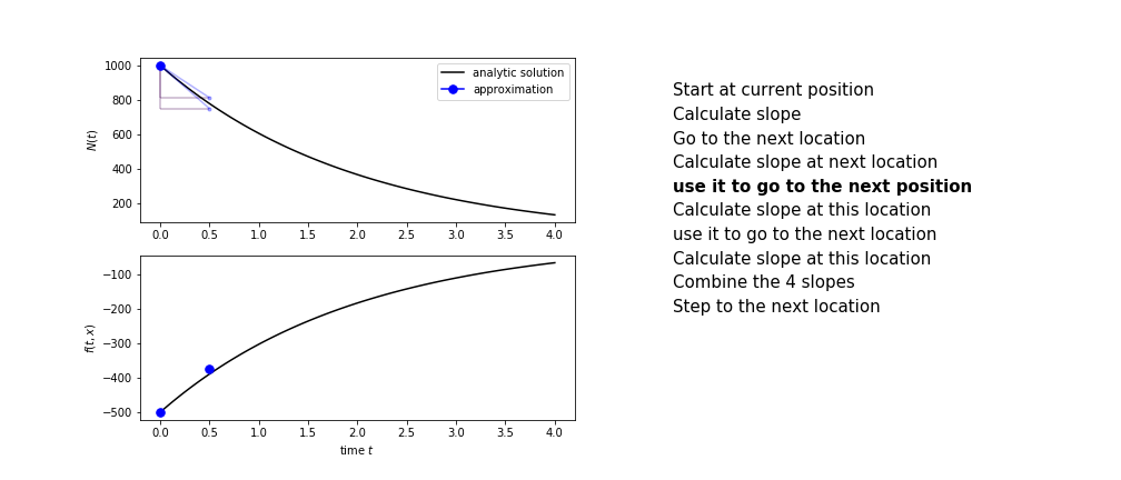
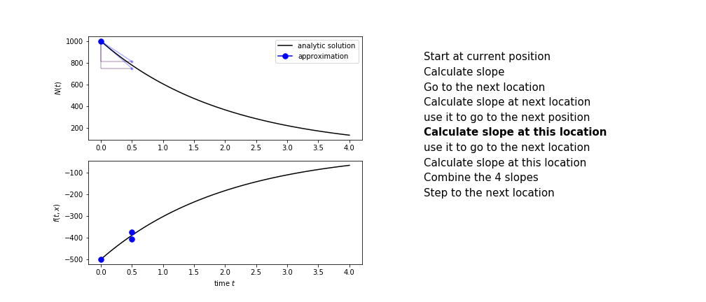
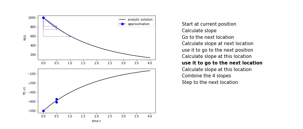
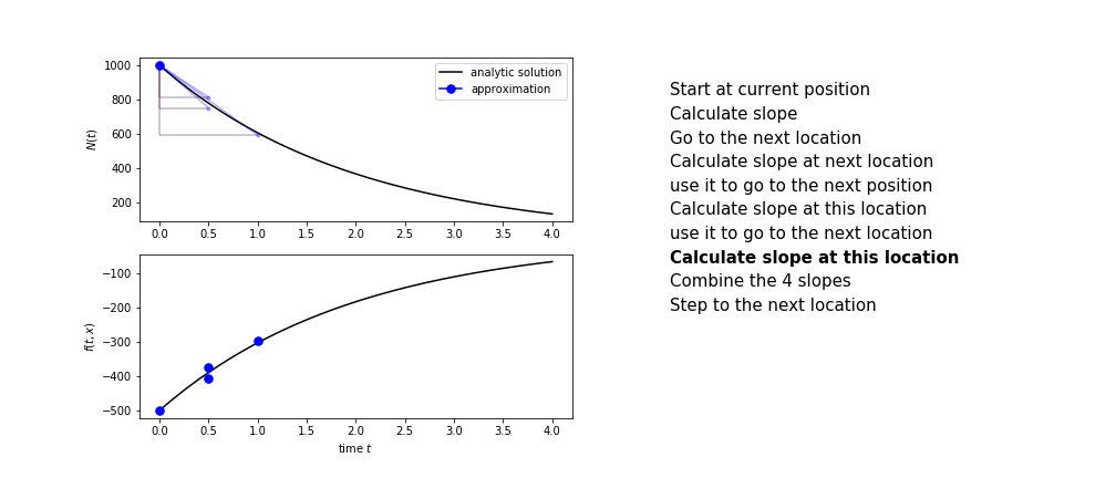
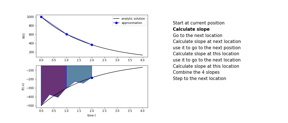
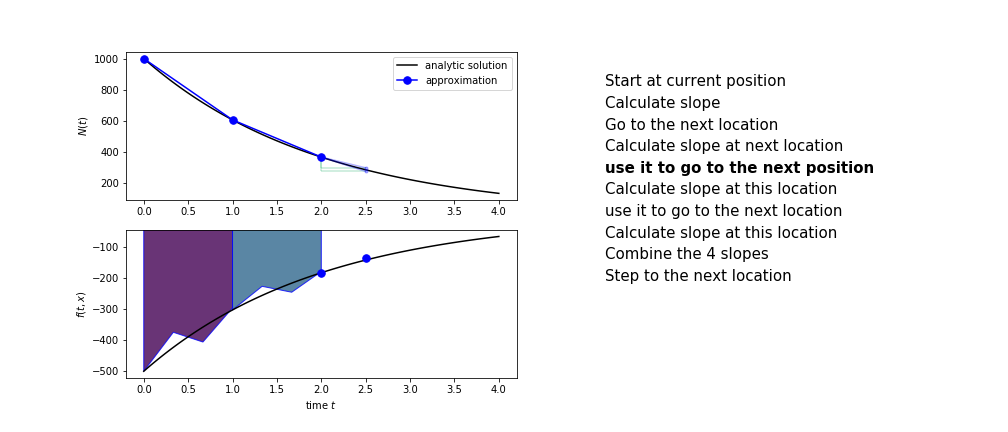
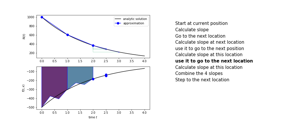
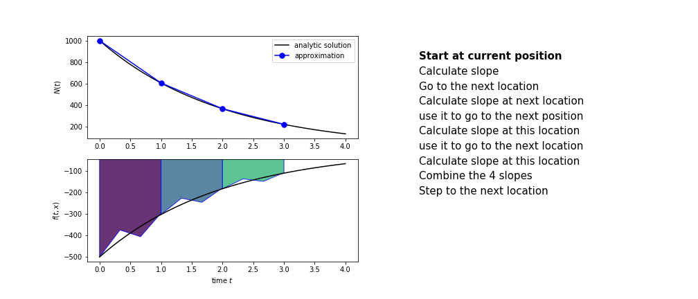
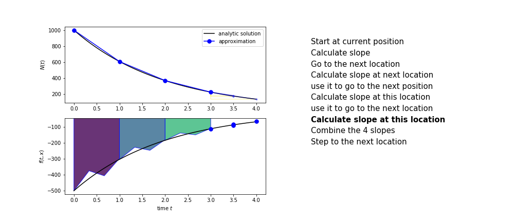
The steps are :
- calculate the slope at the start, call it $k_1$
- use $k_1$ to advance from the start to the middle of the time step interval
- calculate the slope there, call it $k_2$
- use $k_2$ to advance from the start to the middle of the time step interval
- calculate the slope there, call it $k_3$
- use $k_3$ to advance from the start to the end of the time step interval
- calculate the slope there, call it $k_4$
- combine the four slopes as
$$ k = \frac{1}{6}\left(k_1+2k_2+2 k_3 + k_4\right)$$
- use $k$ as the slope to advance to the next step
Runge Kutta 4 demo


Error evaluation
| ODE method | # function evaluations | error per step | total error |
|---|---|---|---|
| Euler | 1 | $\mathcal{O}(\Delta t)^2$ | $\mathcal{O}(\Delta t)^1$ |
| Heun | 2 | $\mathcal{O}(\Delta t)^3$ | $\mathcal{O}(\Delta t)^2$ |
| Runge Kutta 4 | 4 | $\mathcal{O}(\Delta t)^5$ | $\mathcal{O}(\Delta t)^4$ |
The error scaling is shown in this plot.

Assignment 3
You can now finish assignment 3 looking at the radioactive decay using Runga-Kutta method.