Second order differential equations
Second order ODEs
Last week:
$$ \frac{dx}{dt} = f(x(t),t)$$
This week
$$ \frac{d^2x}{dt^2} = f(x'(t),x(t),t)$$
Harmonic oscillator
- mass attached to a string
- pendulum
- electric circuits
- ...
They can all be described with an equation of the form
$$ \frac{d^2 x}{dt^2} = - \omega^2 x $$
We know how to solve 1st order ODE, how do we solve 2nd order ones?
We can decompose the problem into two 1st order ODEs
$$\begin{eqnarray} \frac{dx}{dt} &=& v \\ \frac{dv}{dt} &=& -\omega^2 x \end{eqnarray}$$
They are coupled differential equations:
$$\begin{eqnarray}\frac{d{\bf\color{blue}x}}{dt} &=& { \bf \color{red}v } \\ \frac{d{ \bf \color{red}v }}{dt} &=& -\omega^2 {\bf\color{blue}x} \end{eqnarray}$$
We can use Euler's method to solve it!
Single equation:
$$ x(t+\Delta t) \approx x(t) + \Delta t \frac{dx}{dt} $$
Harmonic oscillator
$$\begin{eqnarray} x(t+\Delta t) &\approx& x(t) + \Delta t \frac{dx}{dt} = x(t) + \Delta t \;v \\ v(t+\Delta t) &\approx& v(t) + \Delta t \frac{dv}{dt} = v(t) - \Delta t \; \omega^2 x \end{eqnarray}$$
Numerical implementation
import numpy
import matplotlib.pyplot as plt

def dx_dt(x,v):
    return v

def dv_dt(x,v):
    return - omgea**2 * x
def evolve(x0, v0, omega, dt, n_steps):
    xs = numpy.zeros((n_steps + 1))
    vs = numpy.zeros((n_steps + 1))
    ts = numpy.zeros((n_steps + 1))

    xs[0], vs[0], ts[0] = x0, v0, 0

    for i in range(n_steps):
        xs[i+1] = xs[i] + dt * vs[i]
        vs[i+1] = vs[i] + dt * (- omega**2 * xs[i])
        ts[i+1] = ts[i] + dt
    return ts, xs, vs
omega, x0, v0 = 1.0, 0.3, 0.1
ts, xs, vs = evolve(x0 , v0, omega, 0.01, 1000)
plt.plot(ts,xs);

Looks good! Let's evolve it a bit more...
ts, xs, vs = evolve(x0 , v0, omega, 0.01, 10000)
plt.plot(ts,xs);

mmmmmm....
ts, xs, vs = evolve(x0 , v0, omega, 0.01, 100000)
plt.plot(ts,xs);

Clearly something is going wrong!
Let's investigate the $\Delta t$ dependence:
for dt in [0.2, 0.1, 0.001]:
    ts, xs, vs = evolve(x0, v0, omega, dt, int(100/dt) )
    plt.plot(ts, xs, label="dt={}".format(dt))
plt.ylim((-10,10))
plt.legend()
plt.xlabel('$t$')
plt.ylabel('$x(t)$');

Is $\Delta t=0.001$ fine?
dt = 0.001
ts, xs, vs = evolve(x0, v0, omega, dt, int(10000/dt) )
plt.plot(ts, xs, label="dt={}".format(dt))
plt.ylim((-10,10))
plt.legend()
plt.xlabel('$t$')
plt.ylabel('$x(t)$');

No! It only takes longer to hit the problem.
The problem:
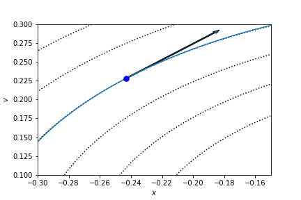
- Inaccuracies of order $\Delta t$ add up!
- look at phase-space to understand the problem
- phase space is the set of possible configuration for the system
Look at phase-space of the system. It is characterised by:
- position $x$
- velocity $v$

For the analytical solution the system moves through an ellipse of constant energy in phase space:
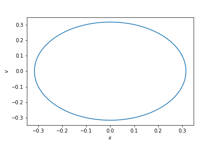
How does it look for the numerical solution?
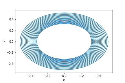
For the numerical solution the energy is not conserved!
Energy is proportional to:
$$ E = v^2 +\omega^2 x^2 $$
After one time step we have:
$$ \begin{eqnarray} E(t+\Delta t)&=& v(t+\Delta t)^2 + \omega^2 x(t+\Delta t)^2 \\ &=& \left(v(t) + \Delta t (- \omega^2 x(t)) \right)^2 + \omega^2 \left( x(t) + \Delta t v(t))^2\right)\\ &=& \left(v(t)^2 - 2 \omega^2 x(t) v(t) +\Delta t^2 \omega^4 x(t)^2\right) + \omega^2\left( x(t)^2 +2 \Delta t x(t) v(t) +\Delta t^2 v(t)^2\right)\\ &=& v(t)^2 + \omega^2 x(t)^2 +\Delta t^2 \omega^2\left( v(t)^2 +\omega^2 x(t)^2 \right)\\ &=& E(t) + \Delta t^2 \omega^2 E(t) \\ &=& E(t) (1 + \Delta t^2 \omega^2 ) \end{eqnarray} $$
We get an exponential growth!
dt = 0.01
ts, xs, vs = evolve(x0, v0, omega, dt, 100000 )
Es = vs**2 + omega**2 * xs**2
plt.plot(ts, Es, label="dt={}".format(dt))
plt.legend()
plt.xlabel('$t$')
plt.ylabel('$E(t)$');

for dt in [ 0.1, 0.05, 0.02, 0.01 ] :
    ts, xs, vs = evolve(x0, v0, omega, dt, int(1000/dt) )
    Es = vs**2 + omega**2 * xs**2
    plt.plot(ts, Es/Es[0], label="dt={}".format(dt))
plt.yscale('log')
plt.legend()
plt.xlabel('$t$')
plt.ylabel('$E(t)$');

Do higher order methods save the day?
Unfortunately not.
- the energy increase at each time step is proportional to
- Euler: $\Delta t^2$
- Heun: $\Delta t^4$
- Runge-Kutta: $\Delta t^6$
regardless how well we estimate the gradient, if we follow it we will land in a place with a larger energy.
Higher orders won't help with this problem. We need to do something else...
Euler Cromer
Implementation Euler
def evolve(x0, v0, omega, dt, n_steps):
    vs = numpy.zeros((n_steps + 1))
    xs = numpy.zeros((n_steps + 1))
    ts = numpy.zeros((n_steps + 1))

    xs[0], vs[0], ts[0] = x0, v0, 0

    for i in range(n_steps):
        vs[i+1] = vs[i] + dt * (- omega**2 * xs[i])
        xs[i+1] = xs[i] + dt * vs[i]
        ts[i+1] = ts[i] + dt
    return ts, xs, vs
Implementation Euler-Cromer
def evolve_EC(x0, v0, omega, dt, n_steps):
    vs = numpy.zeros((n_steps + 1))
    xs = numpy.zeros((n_steps + 1))
    ts = numpy.zeros((n_steps + 1))

    xs[0], vs[0], ts[0] = x0, v0, 0

    for i in range(n_steps):
        vs[i+1] = vs[i] + dt * (- omega**2 * xs[i])
        xs[i+1] = xs[i] + dt * vs[i+1]
        ts[i+1] = ts[i] + dt
    return ts, xs, vs
Now the solution is stable
omega, x0, v0 = 1.0, 0.3, 0.1
ts, xs, vs = evolve_EC(x0, v0, omega, 0.01, 3000)
plt.plot(ts,xs);

omega, x0, v0 = 1.0, 0.3, 0.1
ts, xs, vs = evolve_EC(x0, v0, omega, 0.01, 40000)
plt.plot(ts,xs);

omega, x0, v0 = 1.0, 0.3, 0.1
ts, xs, vs = evolve_EC(x0, v0, omega, 0.01, 100000)
plt.plot(ts,xs);

Error analysis
- we are still making an error at each step
- but now the errors cancel over a period
def analytical(x0, v0, omega,t):
    return x0*numpy.cos(t*omega) + v0/omega*numpy.sin(t*omega)
ts, xs, vs = evolve(x0, v0, omega, 0.01, 10000)
ts, xs_ec, vs_ec = evolve_EC(x0, v0, omega, 0.01, 10000)

ana = [analytical(x0, v0, omega, tt) for tt in ts]
plt.plot(ts,xs-ana, label="Euler")
plt.plot(ts,xs_ec-ana, label="EC");
plt.legend()

This error also increases, but much less dramatically
ts, xs, vs = evolve_EC(x0, v0, omega, 0.01, 10**6)
ana = [analytical(x0, v0, omega, tt) for tt in ts]
plt.plot(ts,xs-ana);

ts, xs, vs = evolve_EC(x0, v0, omega, 0.01, 10**8)
ana = [analytical(x0, v0, omega, tt) for tt in ts]
plt.plot(ts,xs-ana);

ts, xs, vs = evolve_EC(x0, v0, omega, 0.01, 3*10**8)
ana = [analytical(x0, v0, omega, tt) for tt in ts]
plt.plot(ts,xs-ana);
