Notes on queries

A few people seemed to use the analytical solution in their numerical methods.

In real world cases where there is a analytical solution you wouldn't use numerical methods.

The examples we use such as radioactive decay are to facilitate the use of the numerical methods for this course.

This said, some people wanted more Physics examples / questions in these lectures so I've added more in.

Feedback

If you can't access feedback, have any issues please contact me with your CIS username & email me again if I don't get back to you.

Everyone should be familar with the system by now so only extensions from now on via SAC form where your grade will be recalculated from an average of those assignments that you did submit

Assignment 2 Feedback

As with Assigment 1 well answered although some people not reading the question.

I'll upload exemplars for 1 & 2 into the 'Assignment' tab on the website this weekend.

Minor note but on the final version please avoid printing out pages of output.

As with last week some failed the autograder and some plots didn't run!

You can check this with Kernel -> restart & run all.

Plagarism

Need to submit your own work.

You can ask and look stuff up but the blatant copy-pasting is not allowed.

Added a formal plagarism notice in the FAQ section of the website.

Everything you need is on the website, its largely similar assignments every week: implement these equations and plot a graph. Plus, the average mark is quite high so it is clearly very do-able.

I said at the start this isn't a Python course specifically but I'm trying to include Python tips in these lectures. If you don't know something please ask.

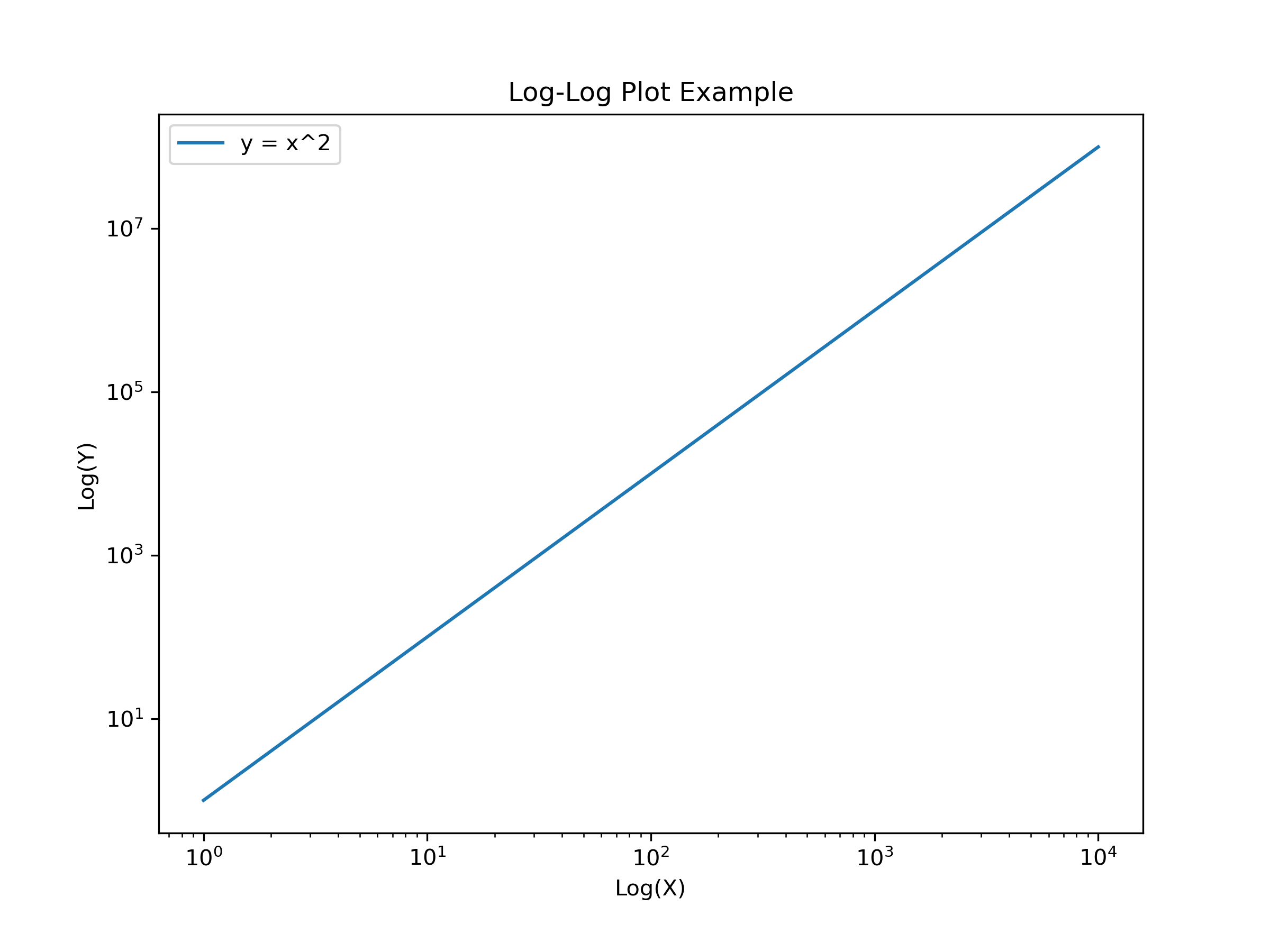
Plotting in Python

                            

# Calculate relationship (marks for this)
x = np.logspace(0, 4, 100)  # 10^0 to 10^4
y = x ** 2  # Quadratic relationship for demonstration

# Create Log-Log Plot (marks for this)
plt.figure(figsize=(8, 6))
plt.loglog(x, y, label='y = x^2')

# Text for graph (marks for this)
plt.title('Log-Log Plot Example')
plt.xlabel('Log(X)')
plt.ylabel('Log(Y)')
plt.grid(False)
plt.legend()

# CHECK THE PLOT IS ACTUALLY CREATED!
plt.show()
                              
                        

Simple Algorithm

Consider a straightforward array update operation.

Maths:

$y(x + \delta x) = y(x) + 2$

Algorithmic Steps:

1. Initialize an array $y$ of zeros with size $n$.
2. Set $y[0]$ to an initial value.

Iterative Update:

$y[x + 1] = y[x] + 2$

Python Implementation

Code Example:

  import numpy as np
  
  # Initialize array and initial value
  y = np.zeros(100)
  y[0] = 1
  
  # Implement Simple Algorithm
  for x in range(99):
    y[x + 1] = y[x] + 2