Generating random numbers according to a probability density

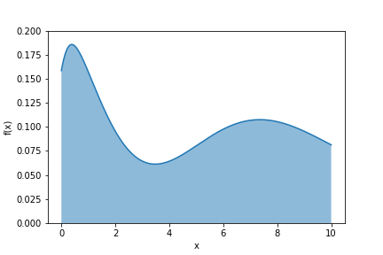
Say we have a function $f(x)$ that describes the probability of a random variable $X$ for taking a value $x$.

How do I simulate values of $x$ that obey that distribution?

Derivation

For a probability distribution $f(x)$ we have:

$$\int\limits_{-\infty}^{+\infty}f(x)dx = 1$$

The strategy is to start with a uniform distribution between 0 and 1 and map it into our new distribution.

Start from a variable $\xi$ that is uniformly distributed between 0 and 1, that is

$$ 1 = \int\limits_0^1 \; 1 \;d\xi $$

Now let's change variable to $\xi = g(x)$:

$$ 1 = \int\limits_{x_0}^{x_1} \frac{d\xi}{dx} \;dx = \int\limits_{x_0}^{x_1} g^\prime(x)\;dx$$

where $g(x_0)=0$ and $g(x_1)=1$.

So to match the definition above we need to have $g^\prime(y)$ match the distribution we want. $$ 1 = \int\limits_{x_0}^{x_1} g^\prime(x)\;dx \qquad\qquad \int\limits_{-\infty}^{+\infty}f(x)dx = 1$$ So if we want values of $x$ distributed according to $f(x)$ our transformation function $g$ will be

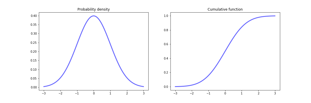
$$ g(x) = \int\limits_{x_0}^x f(x^\prime) dx^\prime $$

This function that integrates the probability distrubution up to a given value of $x$ is called the cumulative function.

Because of the property of a probability distribution function it goes monotonically from $0$ to $1$.

Example of cumulative distributions

Uniform distribution

Normal distribution

Log-normal distribution

Exponential distribution

Generating values

In order to generate values of $x$ we need to invert the relationship

$$\xi = g(x)$$

so we get the recipe :

• generate a value $\xi$ from a uniform distribution between 0 and 1
• calculate the value of $x$ such that $g(x)=\xi$
• this is a new value of $x$
• repeat

Sometimes the inversion is possible analytically, sometimes it has to be done numerically

Example: radioactive decay

The theoretical distribution for the time it takes for a nucleus to undergo a decay of lifetime $\tau$ is given by $$ p(t)= \frac{1}{\tau}e^{-t/\tau}$$

In order to generate decay times according to that distribution we need to calculate the cumulative distribution:

$$ g(t) = \int\limits_{0}^t \frac{1}{\tau} e^{-t^\prime/\tau} \,dt^\prime = 1 - e^{-t/\tau}$$

Now we need to invert the relationship

$$ \xi = g(t) \quad \Rightarrow \quad t = -\tau \ln(1-\xi)$$

This plot illustrates how the procedure works.

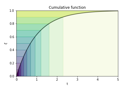Each color band has the same probability of being chosen. By inverting the cumulative function area with the steepest slope (that means the highest probability density) get mapped to narrower ranges of $t$, making these values more likely.

import numpy 
import matplotlib.pyplot as plt

tau = 2.0

xis = numpy.random.random(1000)
decay_times = - tau * numpy.log(1-xis)

ts = numpy.linspace(0,15)
plt.hist(decay_times, bins=ts, density=True);
plt.plot(ts, 1.0/tau * numpy.exp(-ts/tau), 'k--', linewidth=3, alpha=0.5);

xis = numpy.random.random(10000)
decay_times = - tau * numpy.log(1-xis)

ts = numpy.linspace(0,15)
plt.hist(decay_times, bins=ts, density=True);
plt.plot(ts, 1.0/tau * numpy.exp(-ts/tau), 'k--', linewidth=3, alpha=0.5);

The histogram converges to the the right distribution!

Monte carlo hit and miss

Often the probability density $f(x)$ is not integrable analytically so the method outlined before is not applicable.

Another option is to use the Monte Carlo "hit and miss" method.

The recipe is the following:

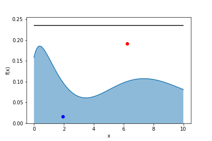
• find a value $m$ for which

$$ f(x)\leq m\;,\;\forall x$$

• repeat:
  • choose a random value for $x$ uniformly
  • pick a random number $r$ uniformly between 0 and 1
  • if $m \cdot r < f(x)$ keep $x$ in the sample ("hit")
  • else discard $x$ ("miss")

Example

Let's look at the following probability distribution:

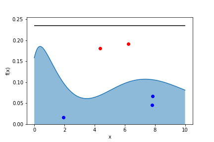
Let's histogram the $x$ values we keep: 1000 tries:

10000 tries:

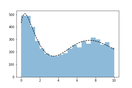
100000 tries:

1000000 tries:

How does it work?

Let's take two values $x_1$ and $x_2$ of $x$. We want the ratio of the probability of $x_1$ being in the sample to the probability of $x_2$ to be in the sample to be equal to

$$ \frac{p(x_1)}{p(x_2)}= \frac{f(x_1)}{f(x_2)}$$

The probability of $x_1$ to be kept in the sample is

$$ f(x_1)/m$$

and that of $x_2$ to be kept is

$$ f(x_2)/m$$

So the relative probability is

$$ \frac{f(x_1)/m}{f(x_2)/m} = \frac{f(x_1)}{f(x_2)} $$

as required.