> Assignments > Assignment 2

Assignment 2

General comments

Overall it was good. The main issues were:

confusion about what the fractional error was and how to calculate it, $\text{abs}((\text{numerical}-\text{analytic})/\text{analytic})$
confusion over how to do a log-log plot.
some students chose unusual log bases (2 or 4) to plot in which wasn’t incorrect, but was impractical as they couldn’t find their power from the slope.
some students enabled xticks in their plots which made their x-axis very difficult to read.
many students had long, wordy titles, often containing phrases like ’log log plot of’ or ‘graph of’.
not giving the power dependence, $1/N^4$ for Simpson’s rule and $1/N^2$ for the Trapezium rule. In the second part we were looking for a comparison. You’ve got the notes to look things like this up.
many students did not understand the round-off error coming from adding small numbers to large numbers meaning a lose of accuracy due rounding of the small number.
many students were confused between the exponential, $e$ , and power laws in their writing.
many students used casual language when describing the errors not related to what is actually happening (e.g. the computer ‘gets in a tizzy’ or ‘can’t cope’ or ‘gives up’)

For the log-log plot there are two possibilities:

plot the log of the quantities on linear axis, in which case state the base you have used, e.g $\log_{10}$ , and you should have log in the axis labels.
plot the quantities themselves on logarithmic scales, in which case there should be no log in the axis labels. The second option is usually preferable as it makes reading the axis more intuitive. To achieve this one can use the

plt.loglog()

call.

Model solution

Automatically marked cells:

def f(x):
    '''Function equivalent to x^2 sin(2x).'''
    return x**2 * numpy.sin(2*x)

def g(x):
    '''Analytical integral of f(x).'''
    return 0.5 * x * numpy.sin(2*x) + 0.25*(1-2*x**2) * numpy.cos(2*x) -1/4

def integrate_analytic(xmin, xmax):
    '''Analytical integral of f(x) from xmin to xmax.'''
    return g(xmax) - g(xmin)

Simpson’s rule can be implemented in a number of ways. Perhaps the most elegant is to create an array of the function values at the end and mid points, an array of the weights for the different points and then multiply them.

def integrate_numeric(xmin, xmax, N):
    ''' 
    Numerical integral of f from xmin to xmax using Simpson's rule with 
        N panels, elegant version
    '''
    xs = numpy.linspace(xmin, xmax, 2 * N + 1)
    ys = f(xs)

    coefficients = numpy.array(( [2.0,4.0] * N) + [1.0])
    coefficients[0] = 1.0
    coefficients[ 2 * N ] = 1.0
    
    panelWidth = (xmax - xmin)/ float(N)
    return 1.0/6.0 * panelWidth * sum( coefficients * ys )

Another option is to have separate arrays of the endpoints and midpoints, sum them and multiply by the coefficients

 def integrate_numeric(xmin, xmax, N):
    ''' 
    Numerical integral of f from xmin to xmax using Simpson's rule with 
        N panels, two arrays version
    '''
    panelWidth = (xmax - xmin)/ float(N)
    xmid = numpy.linspace(xmin+0.5*panelWidth, xmax-0.5*panelWidth, N)
    xend = numpy.linspace(xmin+panelWidth, xmax-panelWidth, N-1)
    total = 4.*sum(f(xmid)) + 2.*sum(f(xend))+ f(xmin) + f(xmax)
    total *= panelWidth/6.
    return total

or create an array of the function values and use an if statement to multiply by the right coefficients.

 def integrate_numeric(xmin, xmax, N):
    ''' 
    Numerical integral of f from xmin to xmax using Simpson's rule with 
        N panels, brute force version
    '''
    # simple brute force method
    xs = numpy.linspace(xmin, xmax, 2 * N + 1)
    ys = f(xs)
    panelWidth = (xmax - xmin)/ float(N)
    # first and last point only have unit weight
    total = ys[0]+ys[-1]
    # loop over all other values (be careful about endpoints)
    for i in range(1,len(ys)-1) :
        # midpoints weight 4
        if i%2 != 0 :
            total+=4.*ys[i]
        # rest weight 2
        else :
            total+=2.*ys[i]
    total *= panelWidth/6.
    return total

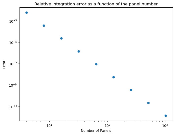
Plotting task

x0, x1 = 0, 2  # Bounds to integrate f(x) over
panel_counts = [4, 8, 16, 32, 64, 128, 256, 512, 1024]  # Panel numbers to use
result_analytic = integrate_analytic(x0, x1)  # Define reference value from analytical solution

errors = []  # Create error array ready for value input 

# For loop generating error data
for n in panel_counts:
    result_numeric = integrate_numeric(x0, x1, n)
    error = abs(result_numeric - result_analytic)/result_analytic
    errors.append(error)

# Log-log error plot
plt.figure(figsize=(8,6))
plt.loglog()
plt.scatter(panel_counts, errors)
plt.xlabel('Number of Panels')
plt.ylabel('Error')
plt.title("Relative integration error as a function of the panel number");

free text questions.

What effect does changing the number of panels used have on the accuracy of the numerical method? What happens if the number of panels is taken too large?

The integration error decreases with $1/N^4$ . If the number of panels is too large we start observing numerical noise from numerical round-off errors.

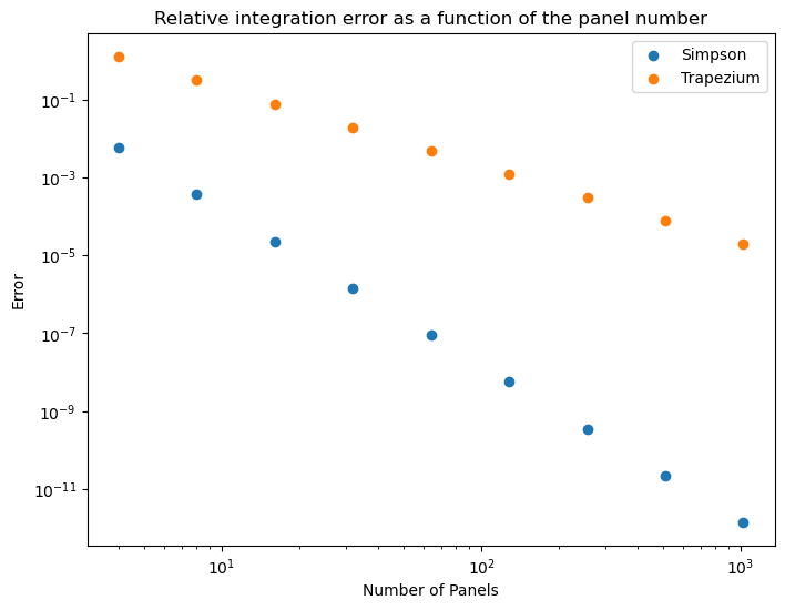
If the trapezium rule was being used, how would the panel count affect accuracy?

The error would only decrease according to $1/N^2$ .

Comparing with the Trapezium rule

So for interest here is some code, and plot comparing the two methods for this integrand.

def integrate_trapezium(xmin, xmax, N):
    ''' 
    Numerical integral of f from xmin to xmax using Trapezium rule with 
        N panels.
    '''
    xs = numpy.linspace(xmin, xmax, N + 1)
    ys = f(xs)

    coefficients = numpy.array([1.0]*(N+1))
    coefficients[0] =  0.5
    coefficients[N ] = 0.5
    panelWidth = (xmax - xmin)/ float(N)
    return panelWidth * sum( coefficients * ys )

x0, x1 = 0, 2  # Bounds to integrate f(x) over
panel_counts = [4, 8, 16, 32, 64, 128, 256, 512, 1024]  # Panel numbers to use
result_analytic = integrate_analytic(x0, x1)  # Define reference value from analytical solution

errors2 = []  # Create error array ready for value input  /mt/home/santoci/

# For loop generating error data
for n in panel_counts:
    result_numeric = integrate_trapezium(x0, x1, n)
    error = abs(result_numeric - result_analytic)/result_analytic
    errors2.append(error)

# Log-log error plot
plt.figure(figsize=(8,6))
plt.loglog()
plt.scatter(panel_counts, errors ,label="Simpson")
plt.scatter(panel_counts, errors2,label="Trapezium")
plt.legend()
plt.xlabel('Number of Panels')
plt.ylabel('Error')
plt.title("Relative integration error as a function of the panel number");

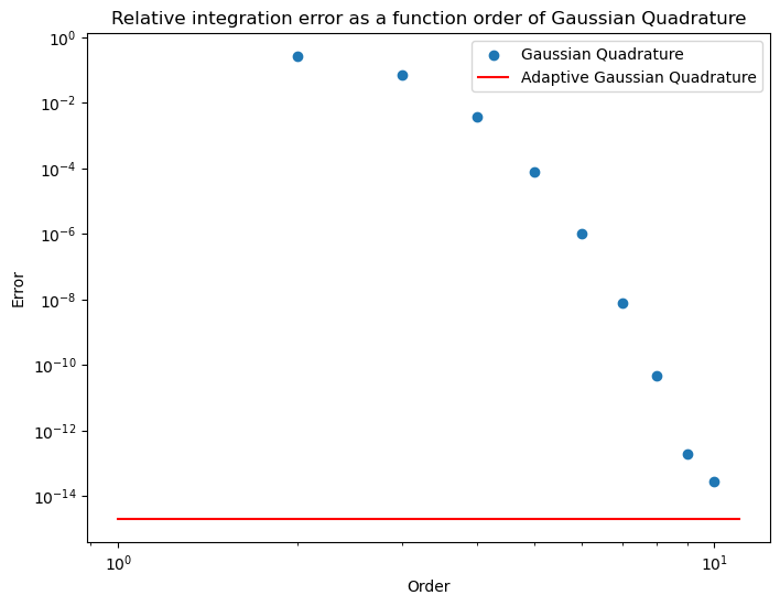
Using scipy

If we really had an integral to do we would not code up the numerical method ourselves. Instead we would use the methods available in scipy. Here’s an example of doing that

import scipy.integrate as integrate

npoints = [i for i in range(2,11)]
error=[]
for n in npoints :
    value=integrate.fixed_quad(f,x0, x1,n=n)[0]
    error.append(abs((value- result_analytic)/result_analytic))
plt.figure(figsize=(8,6))
plt.loglog()
plt.scatter(npoints,error,label="Gaussian Quadrature")

value=integrate.quad(f,x0, x1)[0]
err = abs((value- result_analytic)/result_analytic)
error=[err,err]
plt.plot([1,11],error,label="Adaptive Gaussian Quadrature",color="red")

plt.legend()
plt.xlabel('Order')
plt.ylabel('Error')
plt.title("Relative integration error as a function order of Gaussian Quadrature");